This is the second in a series of posts detailing the application of deep reinforcement learning to radiation source search. In this post, we will cover the theory and basics of reinforcement learning, on-policy deep reinforcement learning, the advantage actor critic, and proximal policy optimization. This post will be heavy on the math but should give some intuition about policy gradients. The first post is found here.

Context

The aim of reinforcement learning (RL) is to maximize the expectation of cumulative reward over an episode through a policy learned by interaction with the environment. In our work, the policy, \(\pi(a_{n+1}|s_{n})\), is a stochastic mapping from states to actions that does not rely on estimates of the state value as required in methods such as Q-learning. We consider radiation source search to be an episodic task which dictates that the episodes are finite and that the environment and agent are reset according to some initial state distribution after episode completion.

On policy, model-free DRL methods require that the agent learns a policy from its episodic experiences throughout training, whereas model-based methods focus on using a learned or given model to plan action selection. On policy methods are worse in terms of sample efficiency than Q-learning because the learning takes place in an episodic fashion, i.e., the policy is updated on a set of episodes and these episodes are then discarded. The benefit being that the agent directly optimizes policy parameters through the maximization of the reward signal. The decision to use model-free policy gradients was motivated by the stability and ease of hyperparameter tuning during training. Specifically, we used a variant of the advantage actor-critic (A2C) framework called proximal policy optimization (PPO).

Reinforcement Learning Preliminaries

The reward starting from any arbitrary time index is defined as,

where \(N\) is the length of the episode and \(\gamma \in [0,1)\) is the discount factor. This definition gives clear reward attribution for actions at certain timesteps and the cumulative episode reward results when \(n=0\).

The agent learns a policy from the environment reward signal by updating its value functions. The value function estimates the reward attainable from a given hidden state that gives the agent a notion of the quality of its hidden state (Sutton & Barto, 2018). This is also a means of judging the quality of a policy, as the value is defined as the expected cumulative reward across the episode when starting from hidden state \(h_{n}\) (will be defined shortly) and acting according to policy \(\pi\) thereafter or more succinctly,

In the previous post, we modeled radiation source search as a partially observable Markov decision process where an observation, \(o_{n}\) is generated at every time step \(n\). We define a history as a sequence of observations up to timestep \(n\), that is defined as \(H_{n}=(o_{0},o_{1},...,o_{n-1},o_{n})\). A successful policy needs to consider \(H_{n}\) to inform its decisions since a single observation does not necessarily uniquely identify the current state (Spaan, 2012). This can be implemented directly by concatenation of all previous observations with the current observation input or through the use of the hidden state, \(h_{n}\), of a recurrent neural network (RNN). The sufficient statistic \(M(H_{n})\) is a function of the past history and serves as the basis for the agent’s decision making (Wierstra et al., 2010). In our implementation, \(h_{n} = M_{\rho}(H_{n})\), where \(\rho\) denotes a RNN parameterization. This allows the control policy to be conditioned on \(h_{n}\) as \(\pi_{\theta}(a_{n+1} \mid h_{n}) = p(a_{n+1},M_{\rho}(H_{n});\theta)\), where \(p\) is some probability distribution, \(\theta\) is some neural network parameterization, and \(a_{n+1}\) is the next action. The expected return of a policy over a collection of histories is then defined as,

where \(\hat{R}_{0}(H)\) denotes the cumulative reward for a history \(H\) and \(p(H \vert \pi)\) is the probability of a history occurring given a policy.

Policy Gradients and the Baseline

Now that we have a formal objective, we can start thinking about how it can be made amenable to optimization techniques. This is where neural network parameterizations come in. We will denote the policy or actor parameterized by a neural network as, \(\pi_{\theta}\), where \(\theta\) are the network parameters. These parameterizations are amenable to first order optimization methods,

where \(\alpha\) is the learning rate, \(k\) is the parameter iterate, and the objective is the expected return of the policy. Equation \ref{eq3} can now be rewritten and we can take the gradient with respect to the parameters to yield,

Several steps have been skipped for brevity but further details can be found in (Sutton & Barto, 2018), (Wierstra et al., 2010). In practice, the true objective is not readily available and so stochastic estimates are used instead that approximate the true gradient in expectation (Sutton & Barto, 2018). We can approximate the expectation through the histories collected by our policy \(\pi_{\theta}\) resulting in the unbiased gradient estimator,

where \(\vert \cdot \vert\) is the cardinality operator. By definition, the gradient of the log probability of the action given the hidden state will be in the direction (in parameter space) that increases the likelihood of that action. Then, we can think of the reward as a scalar component dictating whether to up or down weight the parameters.

Figure 1. Sample of three trajectories plotted over some reward function surface where red corresponds to higher reward and blue corresponds to lower reward. The red square corresponds to the start of the trajectories and the check marks denote the quality of the trajectory where green is the desirable. We want to up-weight the policy parameters that increase the probability of higher reward trajectories occurring and down-weight parameters resulting in lower reward trajectories. This figure was recreated from the following lecture.

A major drawback of the policy gradient approach is the susceptibility to high variance in the gradient estimate due to the computational demand of collecting enough histories to approximate the expectation. Williams proposed the baseline function to reduce the variance of the gradient estimates without adding bias (Williams, 1992). This is represented in the following formula where \(b(h_{n})\) is the baseline function,

An illustrative example of the baseline is to consider an environment where the reward signal is only positive and of varying magnitude. Thus, the gradient step will only be increasing the parameter weights, albeit by smaller or larger amounts. If a baseline such as the sample mean of the cumulative reward across histories of an iterate were subtracted, this would result in the smaller cumulative rewards being negative thereby performing down-weighting those parameters.

Advantage Actor Critic (A2C) and Proximal Policy Optimization (PPO)

A2C

In the A2C framework, the baseline function is chosen to be the value function \(V^{\pi}_{\phi}\) as this captures the expected return from a given hidden state following the current policy. It then becomes immediately clear whether the selected action had a positive or negative impact on the cumulative return and the parameters can be adjusted accordingly. This allows modification of Equation \ref{eq7} to use the advantage function as follows from Schulman et al. (Schulman et al., 2015),

We leave further details to this excellent blog post Schulman et al. propose the following generalized advantage estimator (GAE) with parameters \(\gamma,\kappa\) to control the bias-variance tradeoff,

where \(\delta\) is the temporal difference error defined here. This is an exponentially-weighted average of the TD error where \(\gamma\) determines the scaling of the value function that adds bias when \(\gamma < 1\) and \(\kappa\) that adds bias when \(\kappa <1\) if the value function is inaccurate (Schulman et al., 2015). This leaves the final policy gradient used in our algorithm as,

The value function parameters are updated with stochastic gradient descent on the mean square error loss between the value function estimate and the empirical returns,

Finally, we are ready to discuss PPO.

PPO

A common issue in policy gradient methods is the divergence or collapse of policy performance after a parameter update step. This can prevent the policy from ever converging to the desired behavior or result in high sample inefficiency as the policy rectifies the performance decrease. Schulman et al. proposed the PPO algorithm as a principled optimization procedure to ensure that each parameter update stays within a trust-region of the previous parameter iterate (Schulman et al., 2017). We chose to use the PPO-Clip implementation of the trust-region because of the strong performance across a variety of tasks, stability and ease of hyperparameter tuning as referenced in (Schulman et al., 2017) and (Andrychowicz et al., 2020). The PPO-Clip objective is formulated as,

where \(k\) denotes the epoch index and \(\rho\) is implicit in the hidden state. Here, \(g_{n}(\theta_{k+1},\theta_{k}) = \frac{\pi_{\theta_{k+1}}(a_{n+1} \vert h_{n})}{\pi_{\theta_{k}}(a_{n+1} \vert h_{n})}\), denotes the probability ratio of the previous policy iterate to the proposed policy iterate and \(\epsilon\) is the clipping parameter that enforces a hard bound on how much the latest policy iterate can change in probability space reducing the chance of a detrimental policy update. A further regularization trick is early-stopping based on the approximate Kullback-Leibler divergence. The approximate Kullback-Leibler divergence is a measure of the difference between two probability distributions and the approximation is the inverse of \(g_{n}(\theta_{k+1},\theta_{k})\) in log space. If the approximate Kullback-Leibler divergence between the current and previous iterate over a batch of histories exceeds a user-defined threshold, then the parameter updates over that batch of histories are skipped. OpenAI has an excellent blog post on this topic.

The total loss is then defined as

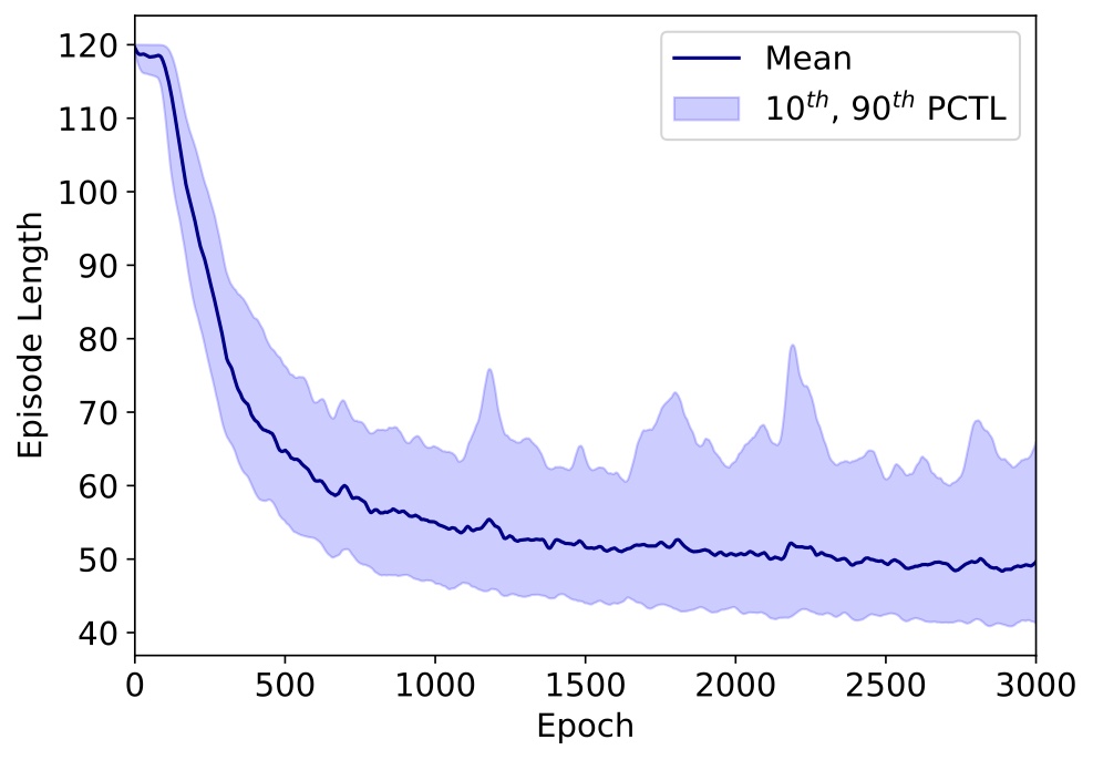
where \(c\) is a weighting parameter and \(\mathcal{L}_{\text{val}}\) is the value function loss. Gradient ascent is performed on this loss to find the set of network parameters that maximize the expected episode cumulative reward. In our work, we plotted the number of completed episodes and completed episode length as performance metrics.

Figure 2. Performance curves during the training process over eight random seeds. The left plot shows the number of completed episodes and the right plot shows the episode length averaged over the 10 parallelized environments per epoch. The dark blue line represents the smoothed mean and the shaded region represents the smoothed \(10^{th}\) and \(90^{th}\) percentiles over the eight random seeds. Episode length decreases and number of completed episodes increases as the model converges to a useful policy. Training for more than 3000 epochs did not significantly improve performance.

Conclusion

This post introduced concepts of reinforcement learning that are fundamental to our approach in solving the radiation source search problem. The key goal of reinforcement learning is learning a policy that maximizes the cumulative episode reward for a given task and environment through trial and error. Radiation source search is framed as a POMDP because the agent only receives noisy observations of the state and thus the agent requires “memory” (hidden state) to be successful. A fundamental component of learning is the value function that provides a measure of the value of hidden states in the environment and thereby enables a principled approach to policy development. By parameterizing the value function and policy with neural network, the reinforcement learning problem can be solved from the optimization perspective, which leads to the A2C architecture. PPO is a further development of the A2C that utilizes a trust region to prevent divergent policy parameter updates. The next post will cover the implementation details the neural network architecture and show some performance results.

1. Sutton, R. S., & Barto, A. G. (2018). Reinforcement learning: An introduction. MIT Press.
2. Spaan, M. T. J. (2012). Partially observable Markov decision processes. In Reinforcement Learning (pp. 387–414). Springer.
3. Wierstra, D., Förster, A., Peters, J., & Schmidhuber, J. (2010). Recurrent policy gradients. Logic Journal of the IGPL, 18(5), 620–634.
4. Williams, R. J. (1992). Simple statistical gradient-following algorithms for connectionist reinforcement learning. Machine Learning, 8(3-4), 229–256.
5. Schulman, J., Moritz, P., Levine, S., Jordan, M., & Abbeel, P. (2015). High-dimensional continuous control using generalized advantage estimation. ArXiv Preprint ArXiv:1506.02438.
6. Schulman, J., Wolski, F., Dhariwal, P., Radford, A., & Klimov, O. (2017). Proximal policy optimization algorithms. ArXiv Preprint ArXiv:1707.06347.
7. Andrychowicz, M., Raichuk, A., Stańczyk, P., Orsini, M., Girgin, S., Marinier, R., Hussenot, L., Geist, M., Pietquin, O., Michalski, M., & others. (2020). What matters in on-policy reinforcement learning? A large-scale empirical study. ArXiv Preprint ArXiv:2006.05990.