This is the first in a series of posts detailing the application of deep reinforcement learning to radiation source search. In this post, we will cover the basics of the nuclear source search task and how we modeled our reinforcement learning environment. Code for the radiation search environment is found here.

Context

The advancement of nuclear technology has brought the benefits of energy production and medical applications, but also the risks associated with exposure to radiation (Sieminski, 2014). Radioactive materials can be used for dirty bombs, or might be diverted from its intended use. Effective detection when these types of materials are present in the environment is of the utmost importance and measures need to be in place to rapidly locate a source of radiation in an exposure event to limit human harm. Autonomous search methods provide a means of limiting radiation exposure to human surveyors and can process a larger array of information than humans to inform the search strategy. Additionally, these techniques can operate in environments where limited radio communication would prevent untethered remote-control of a robot such as the Fukushima Daiichi disaster (Nagatani et al., 2013).

Detection, localization, and identification are based upon the measured gamma-ray spectrum from a radiation detector. Radioactive sources decay at a certain rate which, with the amount of material, gives an activity, often measured in disintegrations per second or Becquerels [bq]. Most decays leave the resulting nucleus in an excited state, which may lose energy by emitting energy-specific gamma rays.
Localization methods in the current work rely upon the intensity in counts per second [cps] of the gamma photon radiation measured by a single, mobile scintillation detector that is searching for the source and is composed of materials such as sodium iodide (NaI). It is common to approximate each detector measurement as being drawn from a Poisson distribution because the success probability of each count is small and constant (Knoll, 2010). The inverse square relationship, \(\frac{1}{r^{2}}\), is a useful approximation to describe the measured intensity of the radiation as a function of the distance between the detector and and source, r.

Figure 1. A mobile robot performing active nuclear source search in a non-convex environment. The source and detector are considered isotropic.

In the case of a single mobile detector, there are numerous challenges to overcome. The nonlinear relationship paired with the probabilistic nature of gamma-ray emission/measurement and background radiation from the environment can lead to ambiguity in the estimation of a source’s location. Common terrestrial materials such as soil and granite contain naturally occurring radioactive materials that can contribute to a spatially varying background rate. 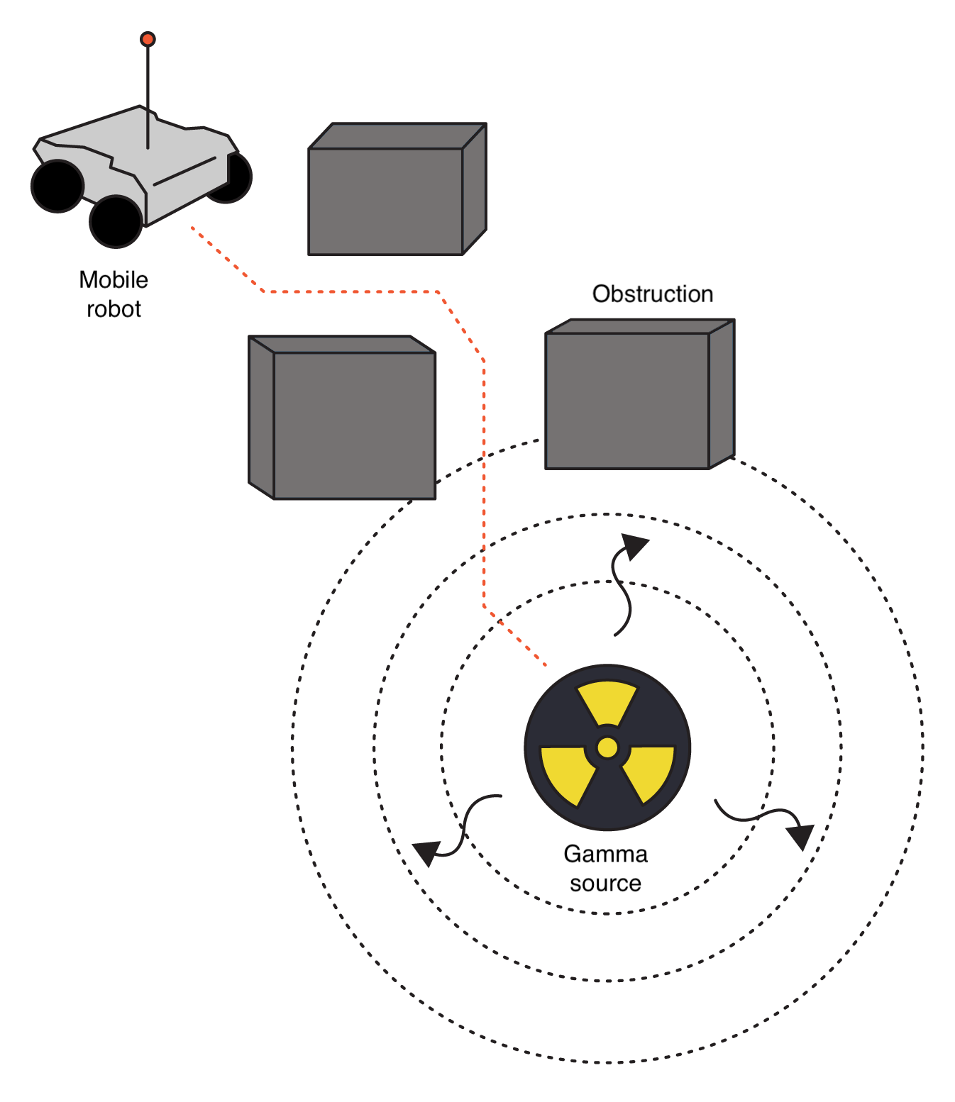Far distances, shielding with materials such as lead, and the presence of obstructions, i.e., a non-convex environment, can significantly attenuate or block the signal from a radioactive source. Further challenges arise with multiple or weak sources. Given the high variation in these variables, the development of a generalizable algorithm with minimal priors becomes quite difficult. Additionally, algorithms for localization and search need to be computationally efficient due to energy and time constraints.

Environment

Gamma Radiation Model

Gamma radiation measured by a detector typically comes in two configurations, the total gamma-ray counts or the gamma-ray counts in specific peaks. The full spectrum is more information rich as radiation sources have identifiable photo-peaks but is more complex and computationally expensive to simulate. Thus, our localization and search approach uses the gross counts across the energy bins. As we are not performing spectroscopic discrimination, our value to describe source intensity \(\mathcal{I}_{s}\) is just gamma rays emitted per second [gps] with the generous assumption of \(100\%\) detector efficiency across the spectrum. We denote the parameter vector of interest as \(\textbf{x} = [\mathcal{I}_{s},x_{s},y_{s}]\), where \(x_{s}, y_{s}\) are the source coordinates in [m]. These quantities are assumed to be fixed for the duration of an episode. An observation at each timestep, \(n\), is denoted as \(o_{n}\), and consists of the measured counts, \(z_{n}\), detector position denoted \([x_{n}, y_{n} ]\), and \(8\) obstruction range sensor measurements for each direction of detector movement. This modeled some range sensing modality such as an ultrasonic or optical sensor. The maximum range was selected to be \(1.1\) m to allow the controller to sense obstructions within its movement step size. The range measurements were normalized to the interval \([0,1]\), where \(0\) corresponds to no obstruction within range of the detector and \(1\) corresponds to the detector in contact with an obstruction.

The background radiation rate is a constant \(\lambda_{b}\) [cps] as seen by the detector. The following binary attenuation model is used to approximate the mean rate of radiation counts measurements when the detector’s line-of-sight (LOS) is or is not blocked by an obstruction,

The measurement likelihood function is defined as

Partially Observable Markov Decision Process (POMDP)

In the context of the radiation search scenario where measurements are noisy and uncertain, it is useful to describe the POMDP. The finite POMDP is defined by the 6-tuple \(\langle \mathcal{S}, \mathcal{Z}, \mathcal{A}, \mathcal{R}, \Omega, \mathcal{T} \rangle\) at each time step, \(n\). The finite sets, \(\mathcal{S}, \mathcal{Z}, \mathcal{A}\), and \(\mathcal{R}\) are states, state measurements, actions, and rewards, respectively. A state, \(s_{n} \in \mathcal{S}\), corresponds to all the components of the environment, some fully observable such as the detector location and range sensor measurements, and others, hidden, such as source activity and source location. A state measurement, \(z_{n} \in \mathcal{Z}\), is the detector’s measurement of the radiation source governed by the state measurement probability distribution, \(\Omega\). A state measurement is a function of the true state but is not necessarily representative of the true state due to the stochastic nature of the environment. An action, \(a_{n} \in \mathcal{A}\), determines the direction the detector will be moved. The reward, \(r_{n} \in \mathcal{R}\), corresponds to a scalar value determined by the reward function. The state transition density, \(\mathcal{T}\), is unity in our context as the state components only change deterministically. An observation, \(o_{n}\), denotes the vector containing the fully observable components of the state \(s_{n}\) and state measurement \(z_{n}\). We define an episode to be a finite sequence of observations, actions, and rewards generated by a POMDP as seen in Figure \(2\). This loop continues until the episode termination criteria is met.

Figure 2. At every timestep \((n+1)\), the agent receives an observation \(o_{n+1}\) and reward \(r_{n+1}\). The observation consists of the fully observable state components and the state measurement, \(z_{n+1}\), that is conditioned on the state \(s_{n+1}\). The observation only gives partial information about the state. The state transition and the reward depend on taking action \(a_{n}\) in state \(s_{n}\).

Gym

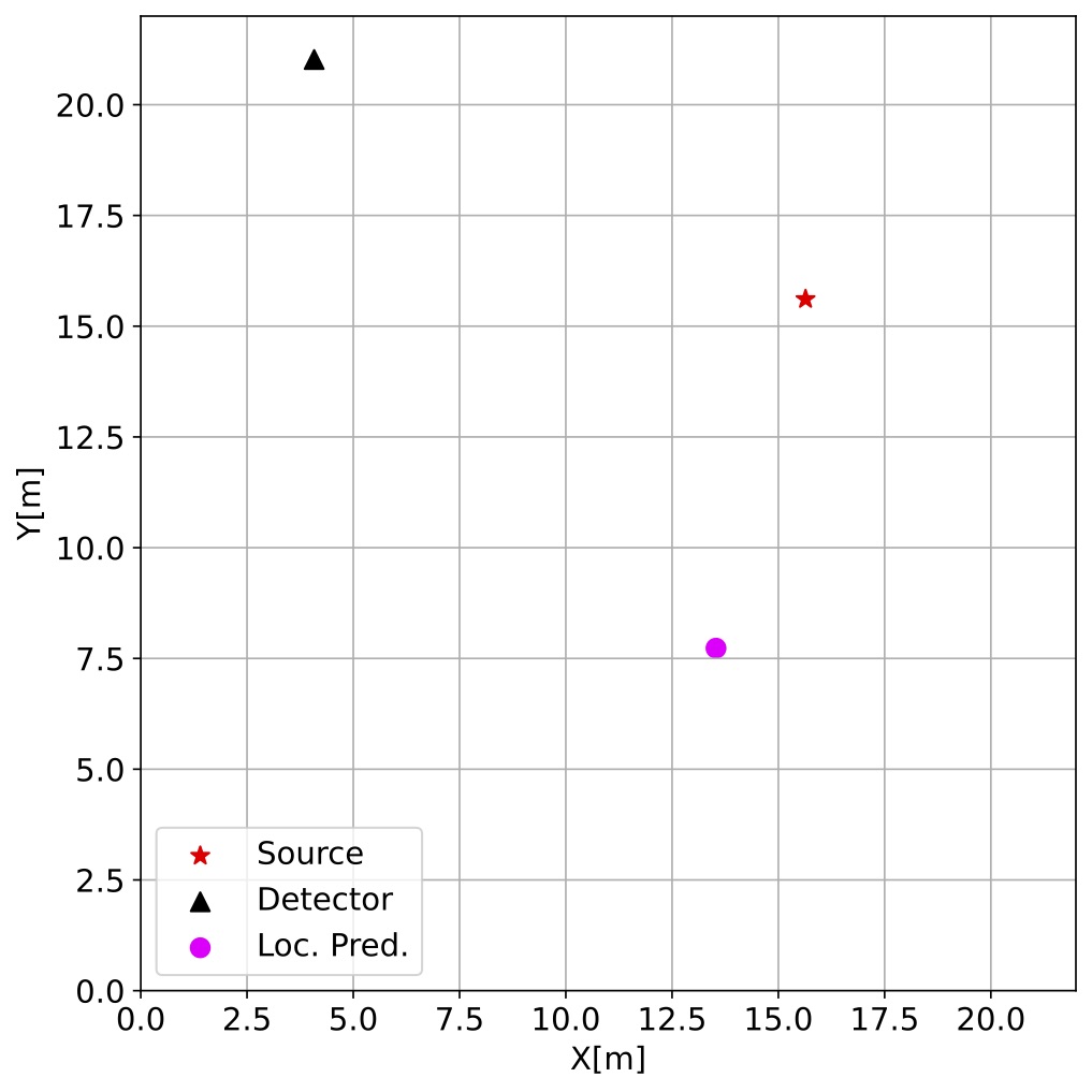
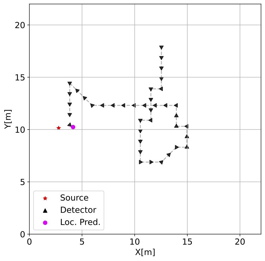
The radiation source search environment was based upon the gym class available in the OpenAI Gym library. Gym is a popular toolkit in the reinforcement learning community that provides a wide array of simulation environments for benchmarking algorithm performance. The main gym class provides a standardized set of methods to codify the observation, action, reward loop of POMDPs (Figure 2). When the radiation source search environment is instantiated, all the parameters are randomly sampled from a uniform distribution. Figure 3 shows two environments with randomly sampled parameters such as source and detector starting position, source intensity, background radiation, and number and location of the obstructions. There is no explicit perimeter boundary constraining the detector.

Figure 3. A sample of the starting conditions for (left) convex and (right) non-convex environments. In both environment types, the red star is the source position, the black circle is the detector position, and the green triangle is the agent's prediction of source position. In the non-convex environment, the gray rectangles are obstructions that block line of sight between the source and detector.

Detector step size was fixed at \(1\) m/sample and the movement direction in radians was limited to the set, \(\mathcal{U} = \{i * \frac{\pi}{4} : i \in [0,7]\}\). Maximum episode length was set at \(120\) samples to ensure ample opportunity for the policy to explore the environment, especially in the non-convex case. Episodes were considered completed if the detector came within \(1.1\) m of the source or a failure if the number of samples reached the maximum episode length. The termination distance was selected to cover a range of closest approaches as the detector movement directions and step size are fixed. The state space has eleven dimensions that include eight detector-obstruction range measurements for each movement direction, the radiation measurement, and the detector coordinates. If the policy selected an action that moved the detector within the boundaries of an obstruction, then the detector location was unchanged for that sample.

Reward Function

The reward function defines the objective of the algorithm and completely determines what will be learned from the environment. Reward is only utilized for the update of the weights during the optimization phase and does not directly factor into the agent’s decision making during an episode. The reward function for the convex and non-convex environment is as follows,

Here, the source-detector shortest path distance is defined as \(\psi\), and \(D_{\text{search}}\) defines the largest Euclidean distance between vertices of the search area. The shortest path distance is essential for the non-convex environment and becomes the Euclidean distance when there is LOS due to the visibility graph implementation. The normalization factor, \(D_{\text{search}}\), in the negative reward provides an implicit boundary to the search area. This reward scheme incentivizes the agent to find the source in the fewest actions possible as the negative reward is weighted more heavily. The reward magnitudes were selected so that standardization was not necessary during the training process as mean shifting of the reward can adversely affect training (Henderson et al., 2018).

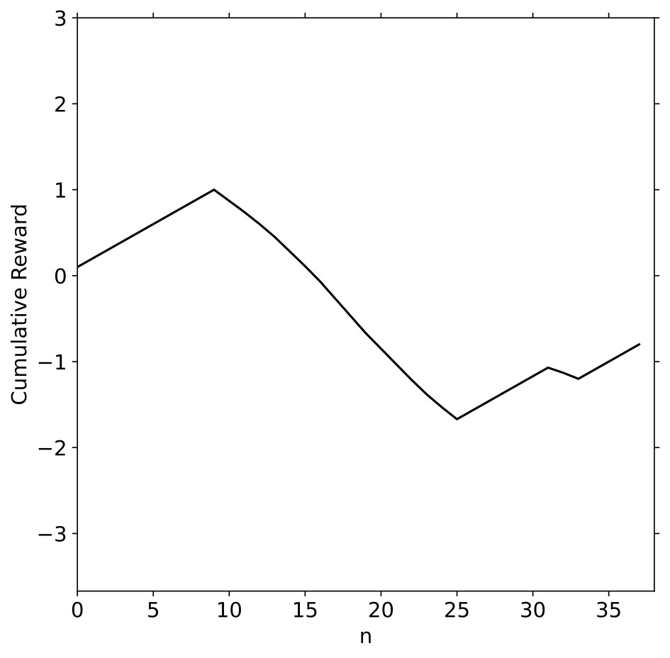
The reward function was designed to provide greater feedback for the quality of an action selected by the agent in contrast to only constant rewards. For example, in the negative reward case, if the agent initially takes actions that increase \(\psi_{n+1}\) above the previous closest distance for several timesteps and then starts taking actions that reduce \(\psi_{n+1}\), the negative reward will be reduced as it has started taking more productive actions. This distance-based reward function gives the DRL agent a more informative reward signal per episode during the learning process. Figure 4 shows an episode of the agent operating within the environment, the radiation measurements it observes, and the reward signal it receives.

Figure 4. Key data streams used by the agent in training and inference. The left plot shows the detector position at each timestep as it moves closer to the source. The center plot shows the radiation counts measurements at each timestep corresponding with the detector position. The right plot shows the cumulative reward signal that the agent uses during training. The reward signal is only used for during training after all episodes in an epoch have been completed.

Conclusion

Radiation source search is a challenging task due to the high variability of the environments being operated in. Many solutions have been proposed for nuclear source search and localization across a broad range of scenarios and radiation sensor modalities. These methods are generally limited to the assumptions made about the problem such as the background rate, mobility of the source, shielding presence, and knowledge of obstruction layout and composition. In the next post, we will cover the basic theory of policy gradients and the deep reinforcement learning technique known as advantage actor critic.

1. Sieminski, A. (2014). International energy outlook. Energy Information Administration (EIA), 18, 2.
2. Nagatani, K., Kiribayashi, S., Okada, Y., Otake, K., Yoshida, K., Tadokoro, S., Nishimura, T., Yoshida, T., Koyanagi, E., Fukushima, M., & others. (2013). Emergency response to the nuclear accident at the Fukushima Daiichi Nuclear Power Plants using mobile rescue robots. Journal of Field Robotics, 30(1), 44–63.
3. Knoll, G. F. (2010). Radiation Detection and Measurement (pp. 73–76). John Wiley & Sons.
4. Henderson, P., Islam, R., Bachman, P., Pineau, J., Precup, D., & Meger, D. (2018). Deep reinforcement learning that matters. Proceedings of the AAAI Conference on Artificial Intelligence, 32(1).